10. View Factors
10.1. The Science Behind : Sky View Factors
10.1.1. A Short History
One of the earliest SVF calculations were made with the help of digital cameras mounted with Fisheye lens. The masks were then delineated manually and the SVF is calculated with Steyn’s method [1]. Other raster-based calculations were later developped, using pixel counting methods [2] [3]. To overcome this somewhat manual and time-consuming method [4]
See also
10.1.2. Sky View Factor and Radiation
A Sky View Factor (SVFs) represents the ratio at a point in space between the visible sky and a hemisphere centered over the analyzed location (Oke 1981) :
At a point where the SVF = O, the entire sky is blocked from view by obstacles. If there is an obstacle blocking parts of the sky view, the SVF will be greater than 0.
for SVF = 0 :
- there is no short-wave reflection
- there is no long-wave nocturnal interference
According to Oke [5], cited by many papers including Hammerle et al. [6], the energy budget (in terms of flux) can in this case be considered ideal
Where Q* is the total energy balance, QGis the energy stored in soil and/or buildings, QHis the sensible heat (air temperature) and QEis the latent heat (evaporated water).
for SVF > 0 :
- incoming day-time short-wave reflection increases during the day
- outgoing night-time long-wave radiation is reduced
- incoming night-time long-wave radiation is increased
- altered soil heat flux
Note
For more information on th different types of radiation, see Night-time Radiation
Because of its influence on energy balances, the SVF holds an importance in various fields of climatology (urban [7], forest [8], human biometeorology [9]...) but its most widespread use concerns the heat island phenomena.
10.1.3. Sky View Factor and Heat Ilsand Phenomena
One of the earliest studies demonstrating the link between sky view factor and local urban temperatures was made by Yamashita et al. [10] (1985).
Footnotes
| [1] | Steyn, D. G. (1980). The calculation of view factors from fisheye‐lens photographs: Research note. Atmosphere-Ocean, 18, 254–258. https://doi.org/10.1080/07055900.1980.9649091 |
| [2] | MMatzarakis, A., Rutz, F., & Mayer, H. (2007). Modelling radiation fluxes in simple and complex environments: Basics of the RayMan model. International Journal of Biometeorology, 51, 323–334. https://doi.org/10.1007/s00484-006-0061-8 |
| [3] | Rzepa & Gromk 2006, Gal et al 2007 |
| [4] | Hämmerle, Gal, Unger, Matzarakis 2001, |
| [5] | Oke, T. R. (1982). The energetic basis of the urban heat island. Quarterly Journal of the Royal Meteorological Society, 108(455), 1–24. https://doi.org/10.1002/qj.49710845502 |
| [6] | Hämmerle, Gal, Unger, Matzarakis, 2011, Comparison of Models Calculating the Sky View Factor used for Urban Climate Investigations, Theoretical and Applied Climatology, Oct. 2011, Vol. 105, n. 3, pp. 521-527 |
| [7] | Watson, I. D., & Johnson, G. T. (1987). Graphical estimation of sky view-factors in urban environments. Journal of Climatology, 7(2), 193–197. https://doi.org/10.1002/joc.3370070210 |
| [8] | Holmer et al., 2001 |
| [9] | Matzarakis, 2001 |
| [10] | Yamashita, 1985, On Relationships Between Heat Ilsand and Sky View Factor in the Cities of Tama River Basin, Japan. Atmopheric Environment Vol. 20, n°4, pp. 681-685 1986 Pergamon Press Ltd. |
View Factors reduce the information given by sky maps and sunny sky maps to a single numerical value, allowing for a more traditional cartography of a discretisized space. Sky View Factors represent the ratio of visible sky at a point, which we could find the Sky View Factor alternatively by attributing to a Sky Map Disc’s center the ratio between the disc’s area and the area representing visual obstacles. Similarily, Sun View Factors can be found by comparing the number of points of a sun path not blocked by obstacles with the total amount of points in the sun path.
10.2. Calculating the Sky View Factor
The Sky View Factor (SVF) is used in the evaluation of the impact of urban geometry on the micro-climate, specifically temperature and the Urban Heat Island phenomenon. Sky View Factors help in the comprehension of an area’s potential direct sunlight in a given amount of time. The SVF indicates the ratio between :
- the radiation received / emitted by a surface from/to the sky
and
- the theoretical total hemispheric radiating environment.
Direct “visibility” between the sky and a plane means radiation can escape the urban setting into the atmosphere, whereas radiation between said plane and another plane keeps radiation trapped. Higher SVFs therefore indicate spaces that would theoretically cool down (emit more radiation towards the sky) than a space with low SVF.
Let’s see how we assess the Sky View Factor in an urban setting. First off, follow the instructions to create a grid layout of the urban space. For this example, we’re using a 10x10 grid, with z=0.1m.
Next, select the Sky View Factor in the BatchProcessing options.
Fill in the next two command boxes accordingly. In the first box:
- Select SkyViewFactor as process
- Select the layer containing your sampled bounding box
- Select “Sketchup:Face”

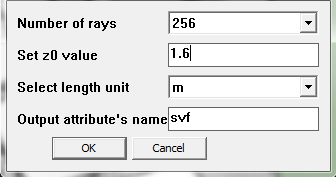
The second command allows you to control the SVF parameters:
- Select the number of rays used to calculated the SVF, ie: its precision. Be careful though, this process is repeated for each sample and will impact your computing time dramatically
- Set the z0 value to 0.1, meaning we will check the SVF at ground level.
- Select your unit length
- Finally, select the name under which the values are stored. We recommend you keep the default name “svf” to keep from any confusion.
Once that is done, you can check your new feature by selecting Extensions > View > PickUpEntity to view individual squares, or by going to Extensions > View > PrintAttributeValues ** and by selecting **svf:Float in the following command box to show the values of every sample.
But there is a much better way of viewing and presenting the data, much like what we’ve done when viewing building heights.
See also
visualizing-bilding-heights
Select Extensions > t4su > View > ColorFaces.
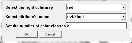
- In the next command box, select the color range you wish to use.
- In the drop-down menu next to “select attribute’s name”, find and select “svf:Float”
- Select the number of classes you want for your map.
- Hit OK
Your grid should be colored to resemble something like this :
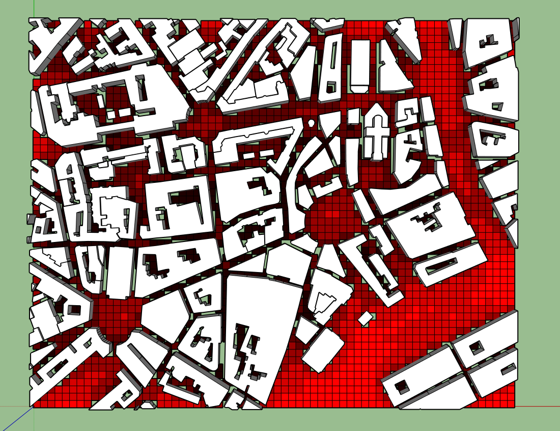
Sky View Factor over Cathedral Sector, Nantes
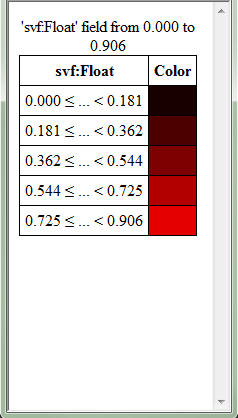
Associated Legend of the SVF Map.
Unless you’ve taken a color range with a “-” in front, lighter values express areas with a high SVF, meaning areas which “view” much of the sky. Darker areas, mostly in small streets and inside building blocks, do not “see” much sky directly : most of the radiation is captured and recaptured by adjacent walls.
10.3. The Science Behind : Solar Radiation
10.3.1. Initial Definitions :
Solar Energy is the amount of energy sent by the sun, meaning the maximum energy received by the Earth, without taking into account climatic conditions (clouds), date or time of day which impact the angle of the surface relative to the sun.
Solar Irradiance (or insolation) is the energy received by a given area of the Earth’s surface. It’s measured in Watts per square meter. As the angle between Sun and surfaces’ normal grows, the solar energy is spread over a larger surface, reducing solar radiance. Solar Irradiation is Solar Irradiance intergrated over time.
10.3.2. Solar Angle and Irradiance
Both place and time come into play when calculating the the solar angle. Place concerns where we are : latitude and longitude :
There are two conjoined earthly movement to be taken into account. - The rotation of the Earth on itself :
- The rotation of the Earth around the Sun :
Finally, we must keep in mind that the Earth’s rotation axe is inclined at 23°27 from the ecliptic plane. This tilt is at the origin of our yearly seasons : we consider the Earth tilted at +23°27 during summer (Souther hemisphere) and -23°27 during winter, the tilt beeing equal to 0 during the equinoxes.
Time concerns The day of the year and the time of day. All of these factors need to be taken into account before any more local analyses.
For Solar irradiation, we need to factor in time :
10.3.3. Atmorsphere’s Interference
Radiation reaches the Earth’s surface in a more or less direct way, depending on the atmospheric interference. Water, dust and pullutants floating in the air will refract rays, dispersing sunlight in multiple directions. The higher the interference, the more diffused the sunlight will be when reaching the surface. The unit of measurement to describe the amount of cloud cover is called an Okta, where 0 Okta is a completely clear sky and 8 Okta is a completely cloudy sky.
10.3.4. Night-time Radiation
Any radiation received by the ground (or buildings) will start releassing heat the moment the air surrounding it turns colder than the soil, typically during night-time.
The radiation emitted has changed to long-wave radiation. In a given urban model, for there to be energy loss (ie, heat loss), the radiation needs to escape back to the atmosphere. This implies a covisibility between the surfaces and the sky vault. More information on Sky View Factor and Radiation
Local weather will greatly affect solar radiation, especially the presence of clouds. As the sun passes through them, the light gets reflected and defused.
10.4. Sun View Factors
Once you’ve created a Sun Path, you can use it to calculate the Sun View Factor, which works a little like the Sky View Factor : instead of checking covisibilities between geometry faces and the sky dome, it will check the covisibility between a geometry and each point of your Sun Path.
Clicking on Extensions > t4su > Sun Views > SunViewFactor will enable the following command box :

- Select the two corresponding layers : your SunPath layer and your geometry layer.
- You can choose to alerate the results slightly by choosing a specific type of sky (from “pure” to “cloudy”).
Once that is done, you will find that your geometries now have extra attributes:
- directSolarIrradiance:Float represents the cumulative theoretical radiative energy received by the geometry from the sun at each point, which depends on their covisibility and the angle of the sun’s rays.*
- nbHitsTotal:Int, the number rays between the geometry and the SunPath points
- nbMinTotal:Float, the number of rays between the geometry and SunPath, multiplied by the frequency of the plot of the Sun Path (eg: for a plot every 5 minutes if nbHitsTotal=2, nbMinTotal=10)
- ratioTotal:Float
You can then use ColorFaces to see the geographical variations of each of these new attributes. Below, we’ve drawn two different maps of the same phenomena : The number of minutes a defined space will receive direct sunlight on two opposing dates : 21st of June and 21st of December, the longest and shortest days of the year respectively.
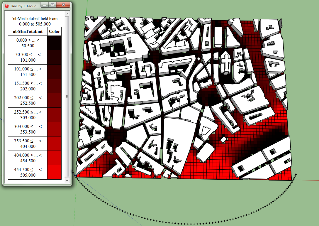
Number of Minutes of Sunlight for the 12st of December
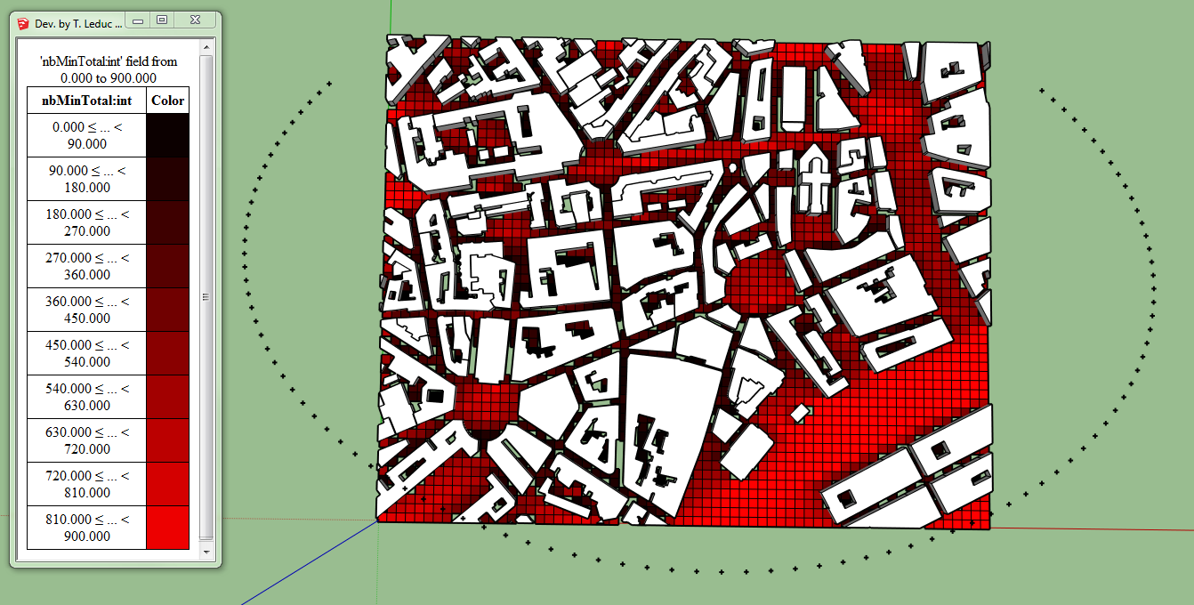
Number of Minutes of Sunlight for the 21st of June
Wouldn’t it be nice to combine these two into a single map, and be able to visualize the difference? Learn how with ArithmeticsOnAttributes.
10.5. Viewing Direct Solar Irradiation along a Path
The city landscaping team has a new shipment of flowers, and they must decide where to plant them. They already have a general idea along a new pathway, using planters that reach two meters high so they can be seen from afar. These plants are very fragile and burn easily in the direct sun.
To find the ideal spot, we first have to recreate the path with line segments that you can import or draw with the SketchUp tool (we will be using the one we’ve used before to explain sampling points). We then proceed to the sampling of line or multi-line into points for example every 5m.
See also
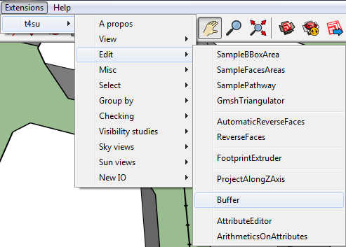
Then, we need to emulate the planters. To do so, we can create a 3D buffer. Click on Extensions > Edit > Buffer
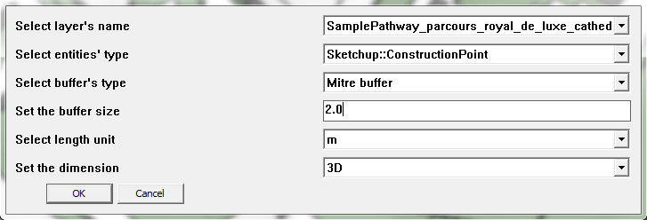
Select the name of the layer containing your sampled pathway and the geometry of the samples (ConstructionPoints). Next, you have the choice to create Round buffers or Mitre buffers (ie, with sharp corners). Select its size : we want 2m because we want to know the conditions at the top of our pedestals, not at ground floor.
Next, we would like to know how much direct solar radiation each pedestal top would receive throughout the year. Create the appropriate sun paths.
See also
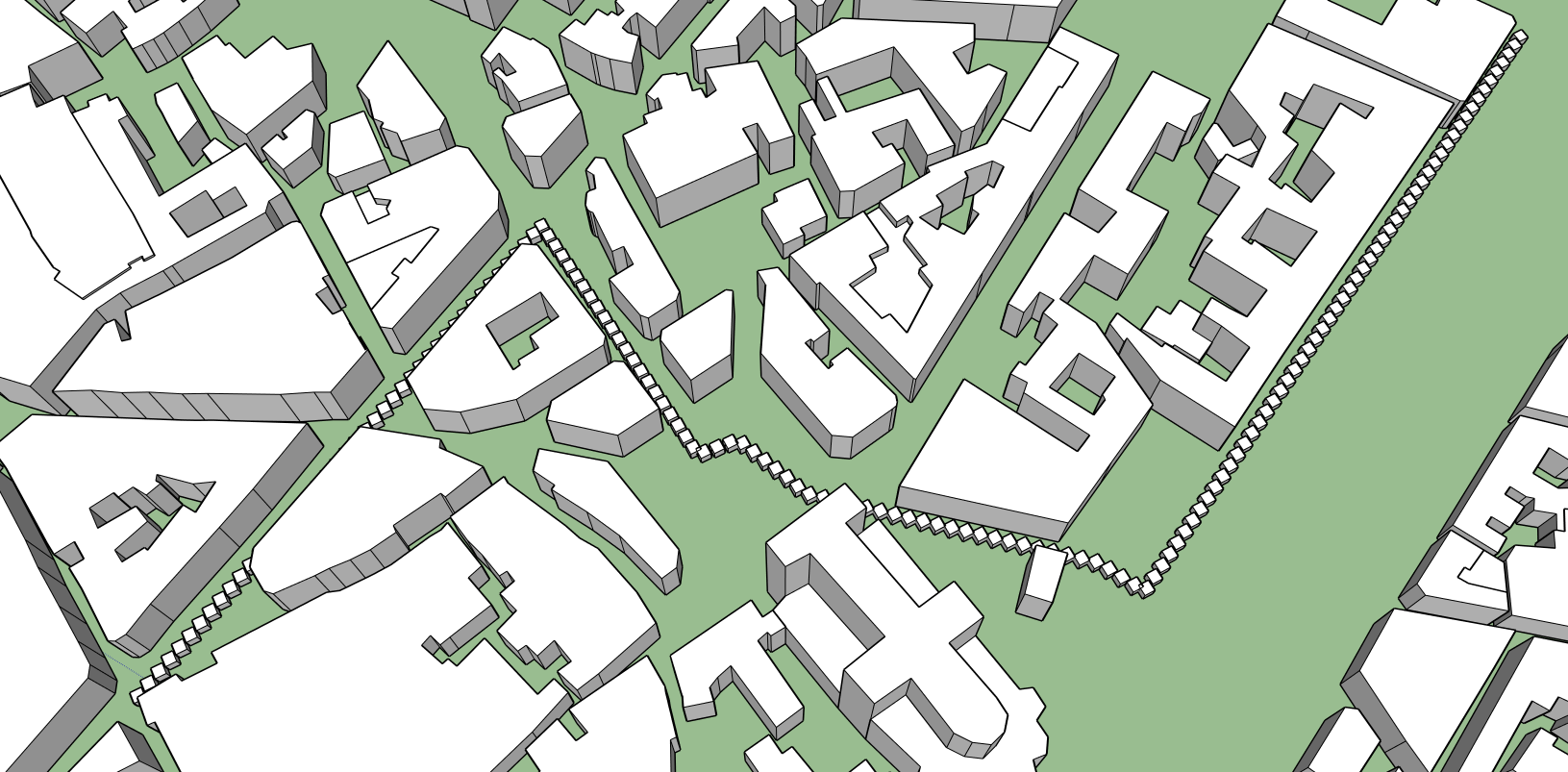
Our plants are here to stay, so let’s create sun paths for the entire year. Go to Extensions > t4su > Select > SelectRoofFaces and select your buffer layer.
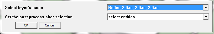
We are finally ready to calculate the direct solar irradiation. Click on Extensions > t4su > Sun views > SunViewFactor. Select your buffer layer in the drop-down list, which still has the “rooftops” selected, as well as your Sunpath layer. You also have the choice of the type of sky. Let’s take the sky will give the highest radiation results : “Pure”. If you click on Extensions > t4su > View > PickUpEntity, you can select each buffer to see the new attributes that have been added. Click on Extensions > t4su > View > ColorFaces and select DirectSolarIrradiance:Float as your classification criteria. You shouldn’t need more than four or five classes. The results show that areas close to intersections generally receive slightly more radiation. It would be best to place the plants along the narrowest streets.
Result of the Direct Solar Insolation along a Path, with Legend.
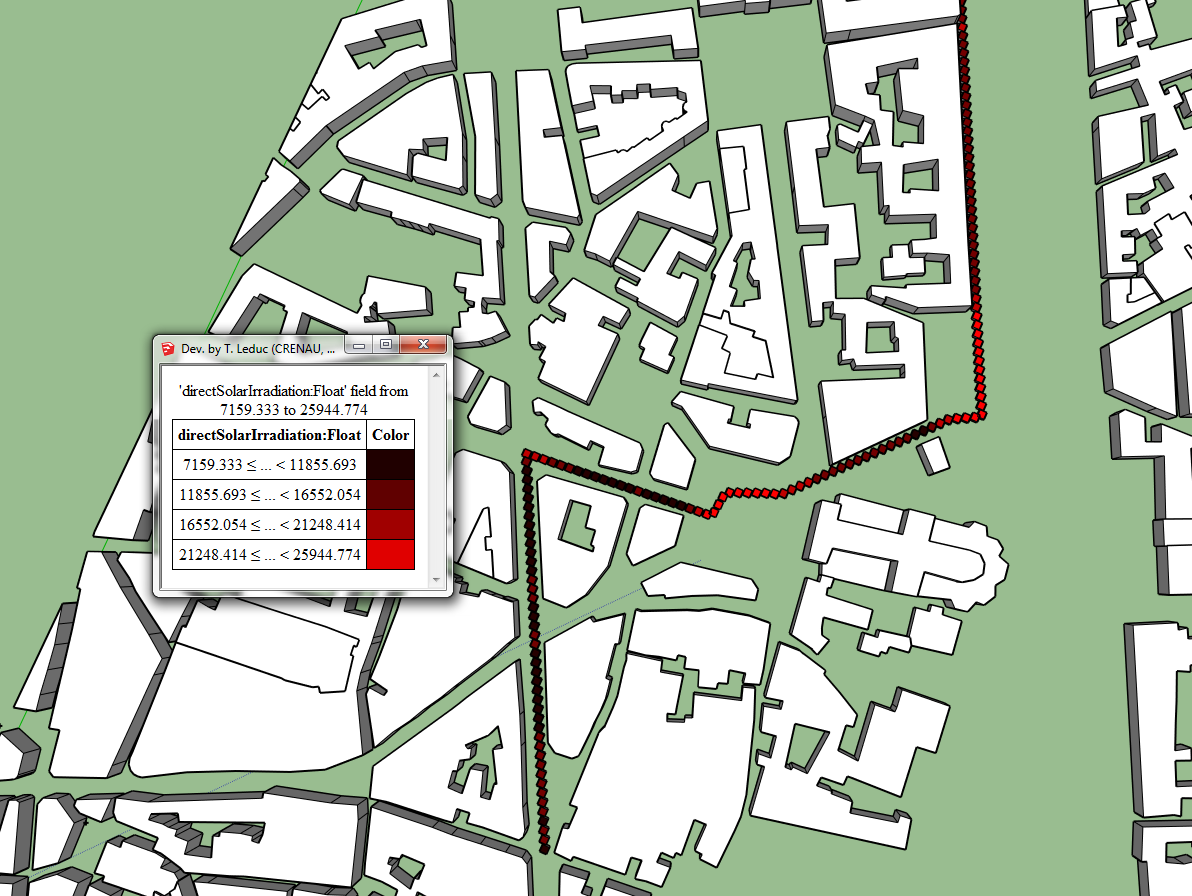
Pinpointed Areas with Least Direct Sunlight, 2m above Street Level.