8. Ray Casting and Isovists
8.1. The Science Behind : Isovists
8.1.1. A Short History
Although isovists are considered to have been first set in theory by Benedikt in 1979 [1] (a first mention of them was made by the same author in 1977 [2]), their first appearance in scientific litterature was a paper by Tandy [3], itself based on writings from on AC Hardy [4]. This concept sprouted from JJ Gibson’s work [5] on “optic arrays”. Benedikt and Burnham [6] give a good explanation of the difference between optic rays and isovists :
- ::
- Imagine a rectangle (representing a room) and the space within it. Draw a straight line between two points on the rectangle; draw another, and another, until the space of the rectangle is effectively filled with criss-crossing lines between all pairs of points. Now chose an point within the rectangle and you find that a large number of lines pass through that point, one of which is shared with another different set of lines passing through a point nearby. If we consider these lines to represent light rays (i.e., photon streams) of varying wavelength and intensity scattered and bounced by the edges of the rectagle (i.e., the walls of the room), then you have an optic array - a set of rays that pass through the point of interest. But where does the otic ray start and end? Is a ray that happens to pass through our point the same ray that it was before it bounced off the wall? If it is, then almost every ray in the room qualifies as belonging to our optic array, as it would eventually pass through our point. Clearly this isn’t going to work. The solution lies in concidering a ray only after its “last bounce”, that is, in concidering only the set of lines – rays – joining our point to the nearest light-scattering surface in every direction. Now, the isovist is simply this optic array, with wavelength and intensity information omitted.
In other words,
- ::
- To every bearing (omega, phi) from a point of observation x in the world there corresponds a distance l, from the point to the nearest surface such that we have a unique ordered set
Several equations derived from isovists and isovist fields (that is, when caculating the isovist for each point in space), mainly from it’s perimeter and area, which an be discretized. We can produce a number of morphological indicators from isovists, including :
- Mean Depth
- Compactness fields
- Occlusivity, occlusivity fields
- Visible Perimeter Fields
Isovist Moments can be derived into three types :
M1 represents represents the derivation from the mean of the perimeter’s distance to x. M2 represented the derivation from the variance of the perimeter’s distance to x. M3 represents the derivation from the skewness of the perimeter’s distance to x. This last formulae can be used to find areas which can see well but
| [1] | ML Benedikt, 1979, “To Take Hold of Space : Isovists and Isovist Fields”, Environment and Planning B, vol 6, pp. 46 - 65 |
| [2] | ML Benedikt, 1977, “Path-dependence and position-dependence in isovist fields”, research report for the Council of Advanced Transportation Studies, University of Texas Austin, Austin, Texas. |
| [3] | Tandy, 1966 |
| [4] | University of Newcastle, unpublished |
| [5] | Lynch 1976 |
| [6] | Gallagher, 1972 |
| [7] | 1966, The Ecological Approach to Visual Perception, Psychology Press Classic Editions |
| [8] | Perceiving architectural space |
8.2. Ray Casting : an Introduction to Visibility Studies
Ray Casting involves choosing a point in your urban space, from which rays will spread at equal distance from each other. The ray stops when it hits either an obstacle or its set limit. It is the simplest and quickest way to assess visibility, but doesn’t give as much information as isovists or hedgehog. First off, click on Extensions > t4su > Visibility studies > RayCasting. A command box will appear, giving you the following possibilities:

Ray Casting Command Box
- Choose the number of rays. This will affect the results’ precision, but taking the maximum isn’t necessarily better : if you select a small visible range, you may not need too many rays.
- The visual range is the maximum length of the rays ; any obstacle after said range will not be picked up during the process
- Set the height (z0 value). If you’re using ray casting for visibility purposes, keep a z-value around eye-level.
- Make sure the units you are working with are correct.
- Finally, you can choose to cast rays in a 2D or 3D space. This is entirely up to the type of information you want to collect. If you are only interested in street visibility and do not need information on the impact of building heights for example, a 2D Ray Casting is much more legible and should suffice.
Once you have click OK, you can click anywhere on your map to cast your rays, as many times as you need (you do not need to repeat the procedure to plot a second RayCast).
2D Ray Casting with 256 rays at a distance of 40m
2D Ray Casting with 1024 rays at a distance of 150m
If you are not interested in the rays themselves, but rather the point of impact they share with the facades of your buildings, check out CloudOfPoints.
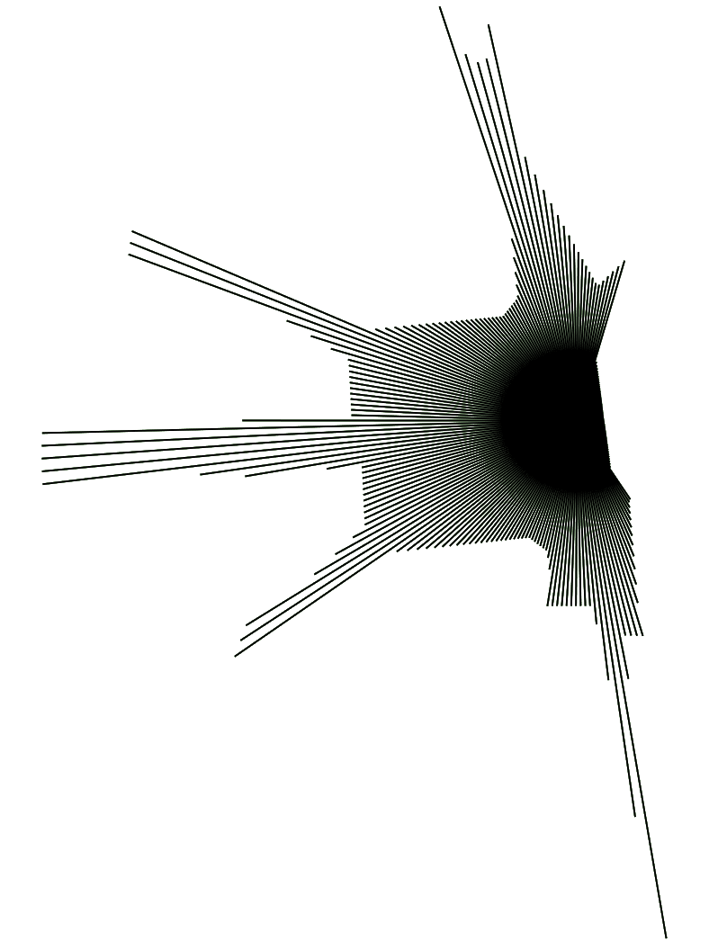
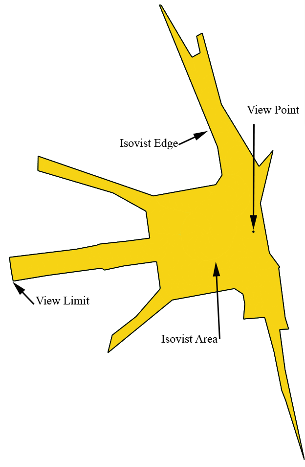
8.3. What is an isovist ?
Isovists represent the entirety of the visible plain (in 2D) or volume (in 3D) at a specific point in space, bounded by the built environment. Because isovists are built upon a point, the associated form changes as it is displaced, just as our notion of urban space changes as we walk through it. They are frequently used in many fields of visibility studies : wireless network design, landscape management and analysis, pedestrian access or security.
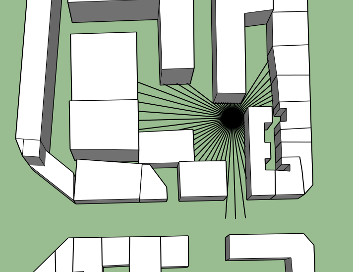
Isovist at a Point Close to the Cathedral.
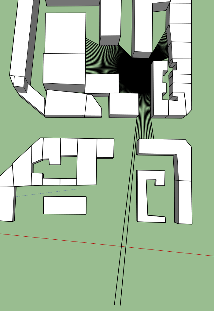
Isovist at an Other Point in Space.
So how are isovists built? Originating from our point of origin (view point), rays are cast into the open space, up to a certain arbitrary distance (view limit). The resulting points of impact between each ray and its barriers (either obstacles or the view limit) are joined to form the isovist’s edge. The rays are then replaced by an isovist area.
Isovists can also be used to study a space’s convexity, that is, a region for which every pair of points in said region can be linked by a straight line also within the region. Here is a simple example of convex and non-convex spaces:
In a Convex Space, Isovists have the Same Shape no Matter the Location of the View Point
In a Non-Convex (Concave) Space, more than one Isovist is Needed to Map the Totality of the Area.
We can notice the link between ray casting and isovist formation when playing with its precision.
8.4. Creating Partial 2D Isovists
Partial isovists are isovists that are constrained by a certain aperture. You can automate their process using BatchProcess, or set your positions and orientation manually by clicking Extensions > t4su > Visibility Studies > PIsovist 2D. If you’re using the manual method, you will be redirected to the Partial Isovist Command Box.
First, import a linear geometry (ie: made of lines or multilines) into your Layers, or draw one yourself using the Line Tool.
See also
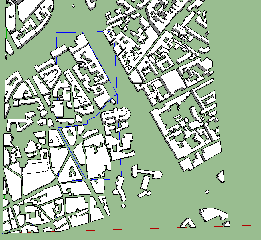
Next, you’ll want to sample your pathway, then use a Batch Process.
Select PIsovist2D (which stands for Partial 2D Isovist) in the Process to apply and select the correct layer (starting with SamplePathway[...] if you’ve created your points through sampling). Finally, select Sketchup::ConstructionPoint as Geometry type.
If don’t want to use a Batch Process or would rather select the points manually,you can do so too. Simply click to set the point of origin and drag to set the orientation of your partial isovists.
Whether you’re plotting manually or automatically, you will have to fill in this command box :
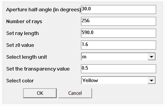
- Select the aperture of your circular sectors (ie: how wide you wish the isovist to be)
- Select the number of rays : a higher number will give a more precise outline, but a lower number will greatly accelerate computation time. For example, setting the aperture to 30 and the number of rays to 60 will result in a ray every 0.5 degrees.
- Select ray length. Some trial-and-error may be needed to adjust this parameter : too short, they may not cover enough ground. Too long will result in confusing overlapping geometries and longer computation times.
- Setting the z0 value allows you to decide at which height the partial isovists are calculated. By default, they are at 1m60, an average person’s eye-height.
- You may also change the appearance of the isovists : transparency (from 0 to 1, 1 being the most opaque) as well as the color.
- When you are ready, click OK
What do we see ?
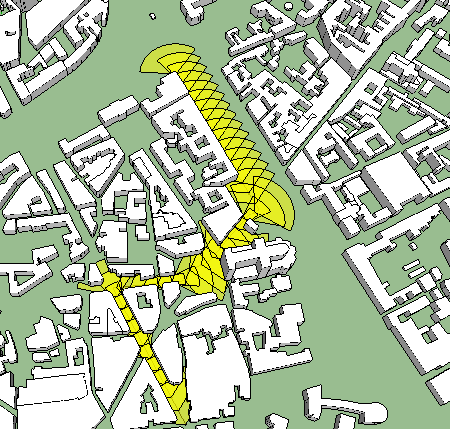
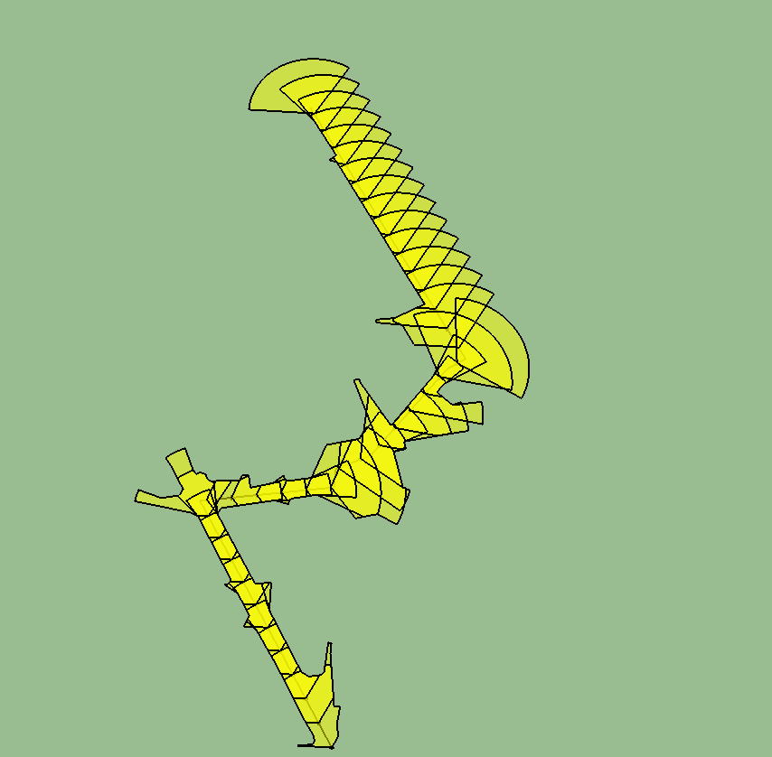
The partial isovists are constrained by the extruded building geometries. Their profile mimics our visibility as we advance along the path we have decided upon. We can notice the gradual enlargement of the isovist as we advance towards an plaza or an intersection.
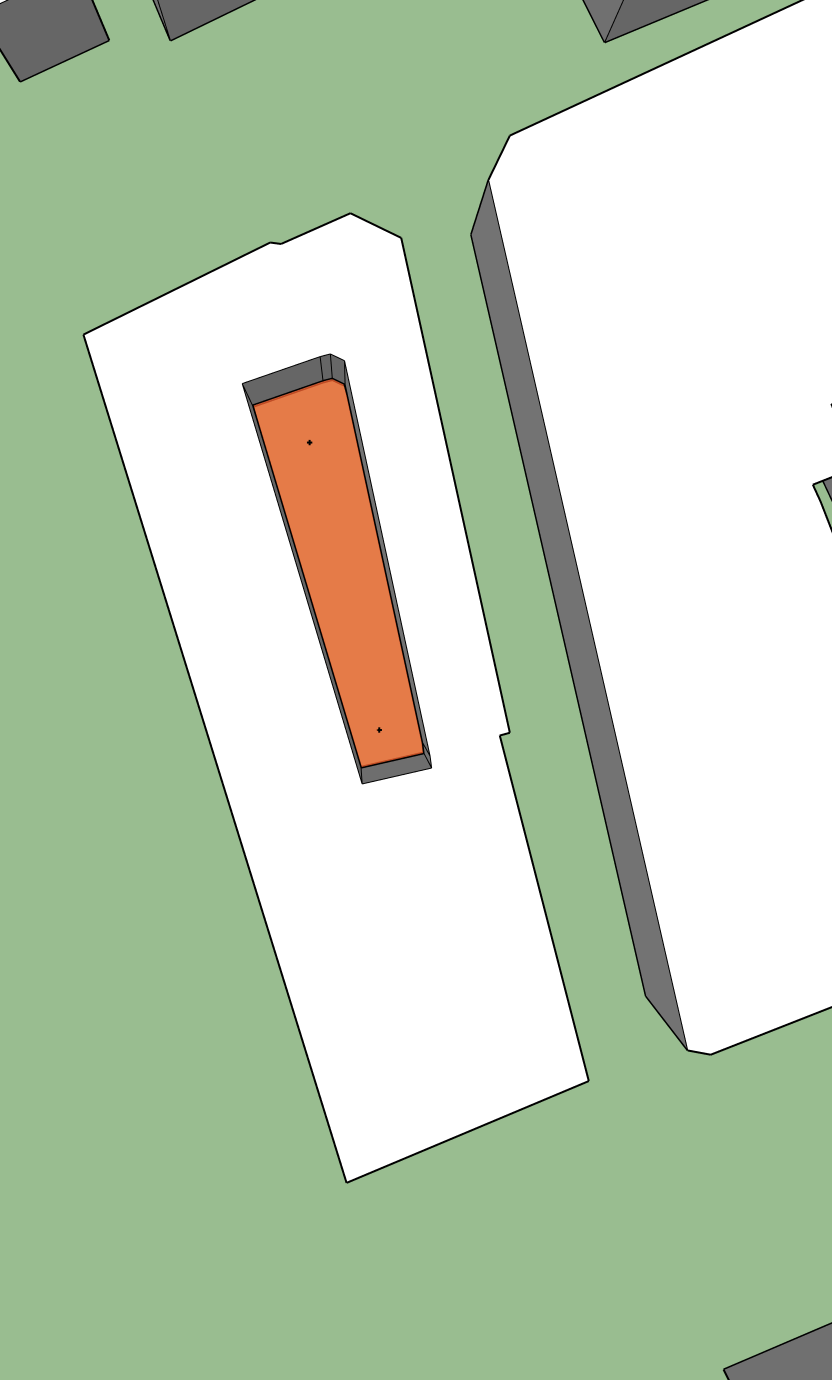
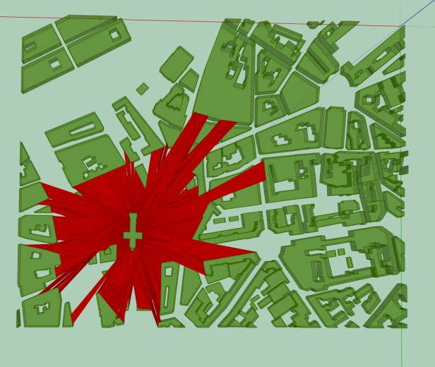
8.5. 3D Isovists and Hedgehogs
Like 2D Isovists, 3D Isovists and hedgehogs use ray casting to map the surrounding urban space. Unlike it’s 2D counterpart though, 3D Isovists will only output assembled rays that effectively touch a surface.
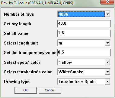
Isovist Command Box
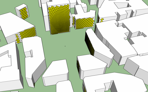
When creating these 3D objects, you will have to decide whether to draw “tetrahedra or spots” (or both). By choosing tetrahedra, the cast rays are drawn, set in a group and shown. Spots on the other hand, draw out the surfaces visible from our point of interest (i.e., the faces’ areas touched by the tetrahedra).
3D Isovist, Spots Only
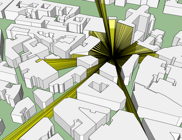
3D Isovist, Spots and Tetrahedra
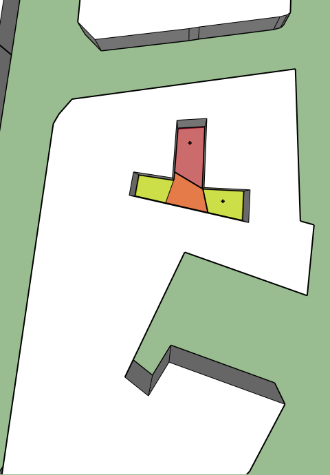
The surfaces are created by a minimum of three points, meaning if only two rays reach a surface, that surface will not be taken into account in the Isovist/Hedgehog rendering. You will also get the following error:
The difference between a hedgehog and a 3D isovist lies in whether or not these batches of three rays form individual tetrahedra/spots, or are assembled into one. Here’s an illustration of a Hedgehog result: compare it with the Isovist result above (resolution was slightly lowered).
Hedgehog Result, Spots Only.
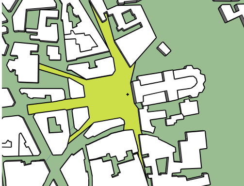
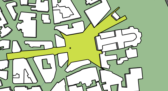
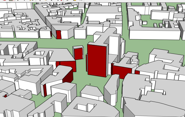
As with many other features, it is possible to run a batchprocess of 3D isovists. In this last example, the cathedral building wall faces were selected and sampled into points. The following result allows us to know which building facades have a potential view of any side of the cathedral.
Building Facades with Direct View of the Cathedral