5. General Tips to Start
T4SU offers many features that allow for an automatic selection, modification, creation or visualization of information, for a fast and easy way to treat and analyse our data. Many of these techniques will be used again in examples throughout the manual.
5.1. Selecting Geometries
One of the many features of T4su is that it will automatically recognize selected objets when running a process over a layer, and will run that process only on the selection. So if you want to run a process on an entire layer, make sure to not have anything selected. The T4su extension includes a very extensive assortment of selection tools, each oriented towards a specific usage. You can find this collection when clicking Extensions > Select. Regardless of the type of selection, you will have the same three post-process after selection choices:
- simply selecting the geometries;
- automatically deleting the geometries;
- moving the geometries to a new layer. The layer will be named [NameOfSelectionProcess]-[Date and Time]
5.1.1. Types of Selection Processes :
- SelectRoofFaces : this will select the top-most geometries
- SelectWallFaces : this will select all the vertical faces.
These two selection features are pretty good at distinguishing one from the other. To test this, I’ve modified my original shapefile, adding a pointed roof and a small dormer on top of the original roof. The selection module still works :
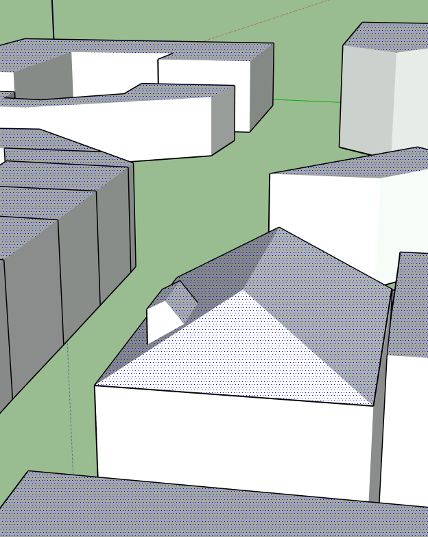
Roof Selection
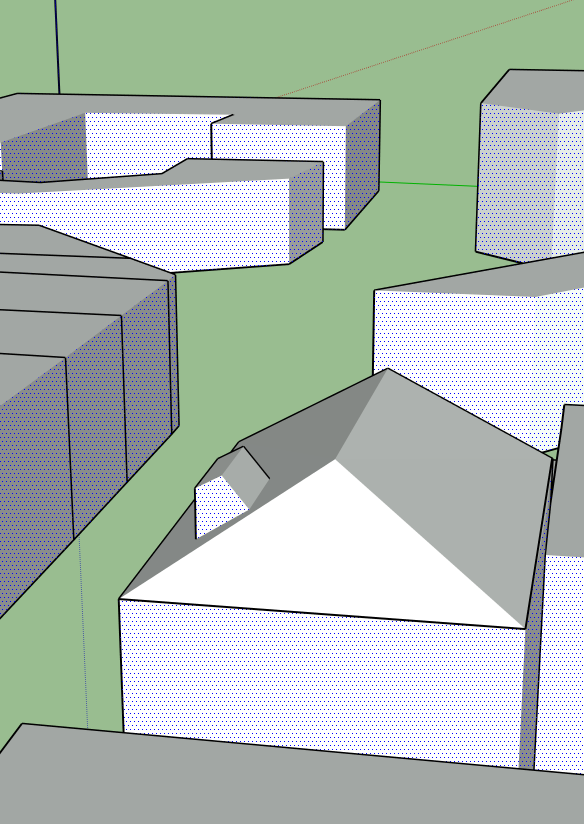
Wall Selection
- SelectGroundLevelFaces : Selects all the faces with a z0 value of 0. When performing this on a building layer, this selects the ground floor. This will also work for ground-level Sampled Faces and Bounding Box with a Z-value of 0.
- SelectAllConnectedFaces : used for export towards Salome
- Select UnnecessaryEdges : selects Tin edges of coplanar surfaces to simplify a rough terrain by grouping coplanar faces. This is mainly used used directly with the remove geometries option. You may have to play around with the threshold value, as there’s a strong chance some of your faces will disappear. This is because your threshold value is too low, meaning your margin of error is too large when selecting coplanar faces. Conversely, choosing too small a value will hardly reduce your number of faces, if any at all.
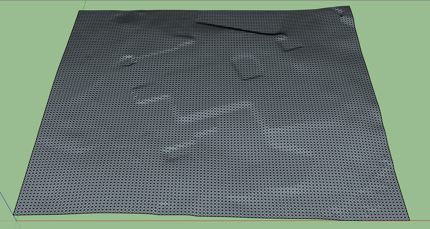
Original Terrain
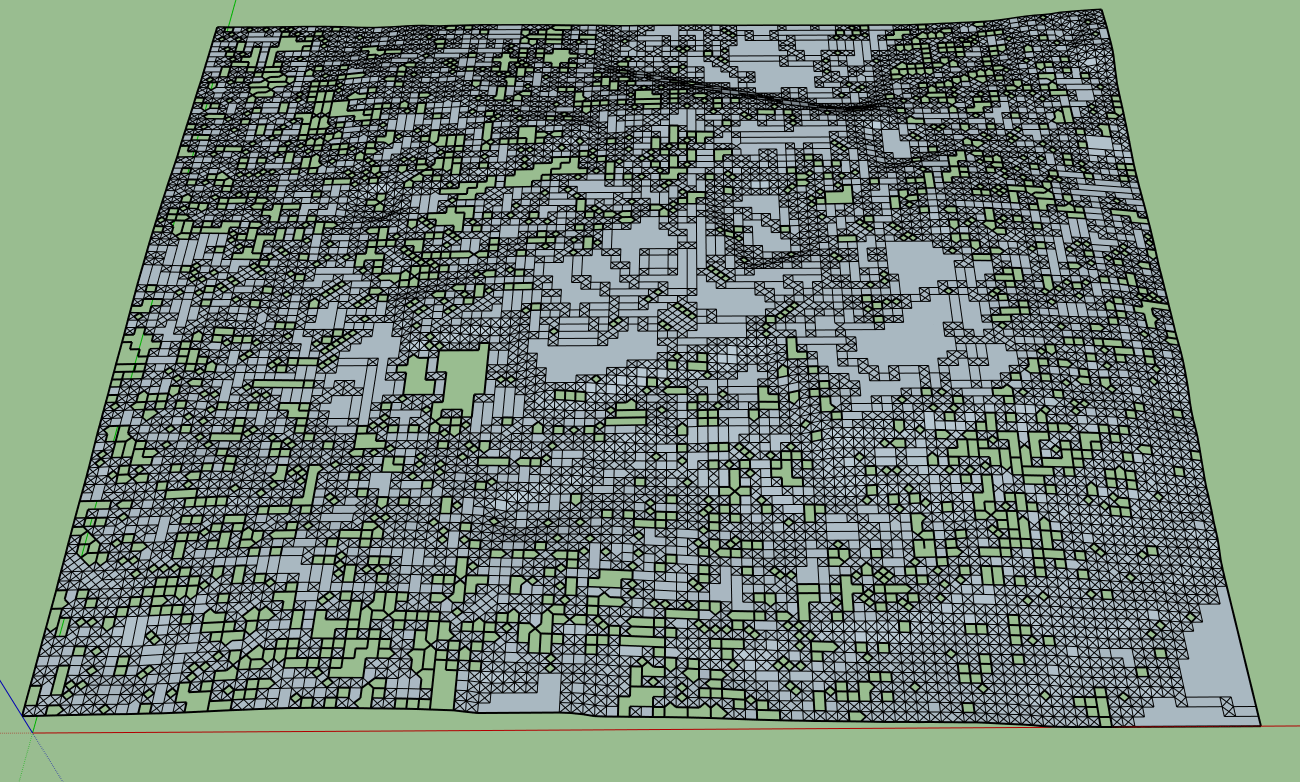
Deleting Unnecessary Edges with Too Low a Threshold will Puncture the Terrain
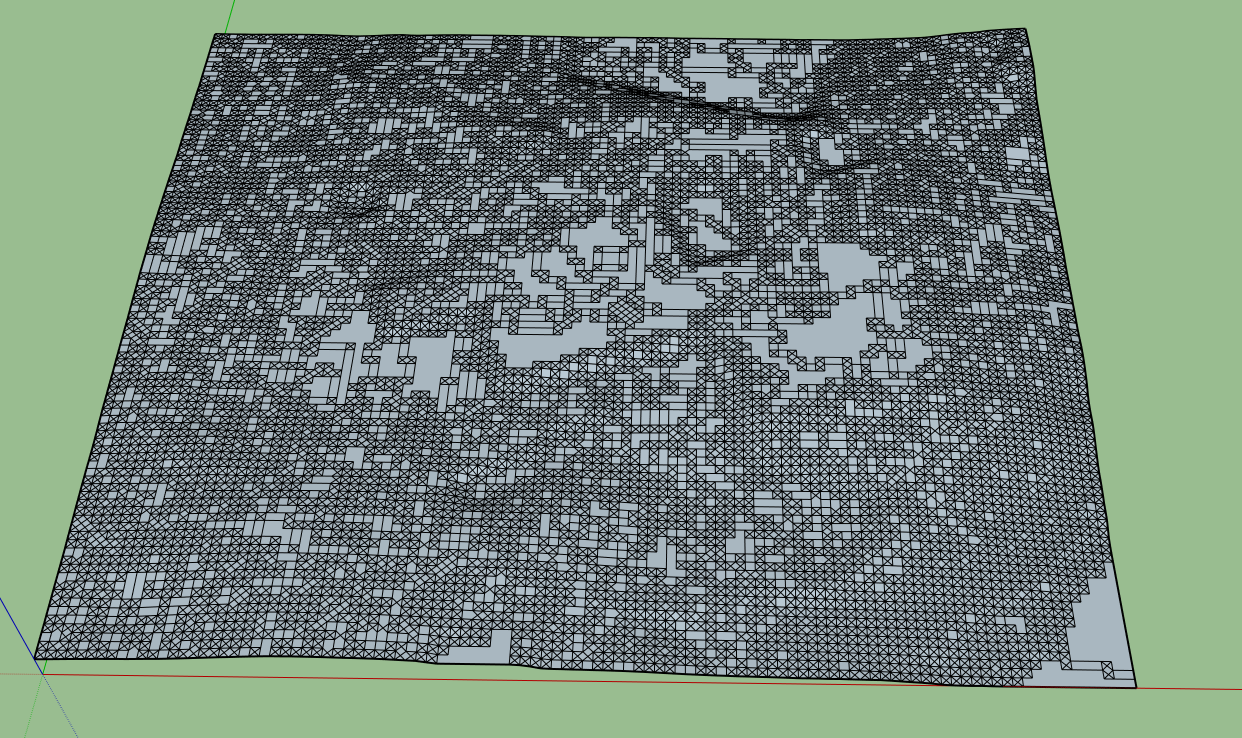
Result of Selecting a Correct Threshold for Unnecessary Edges
- SelectGroupsAccordingToVolumeProperties : Whether the 3D geometry is closed (ie, hermetic, bounded by faces on all sides), or open (missing a face, or with window or door openings).
An interesting feature is that these types of selections will bypass geometry Groups made in sketchUp.
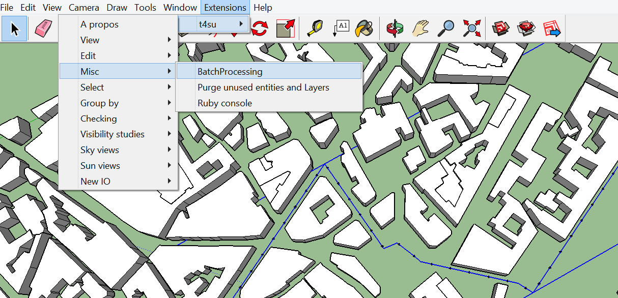
5.2. Batch Processing
Batch Processing allows you to automate a number of processes available in t4su, rather than working with point-and-click.
You first need to plot any points of interest, through a sampling method, or by importing a layer or geo-localized points. Using predefined data for your calculations allows for a more precise result than using your mouse for each individual point, and may be time-saving depending on the number of points you have.
Once you click Extensions > Misc > BatchProcess, the following box will appear :
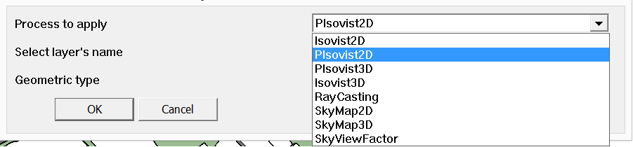
Select your layer containing your data points. These will be at the center of your disks (if you work in 2D) or spheres (for 3D Isovists or Sky Mapping), or the origin of your rays (in the case of Ray Casting).
5.3. Running Times and Geometrical Precision
Most modules in T4SU allow you to choose your precision. There are general guidelines for choosing the correct. First, we can notice that the precision “p” follows the equation:
What is the concrete impact of augmenting precision ? Here is a first concrete example using 3D Sky Map:
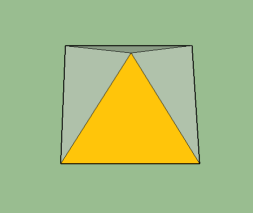
3D Skymap (p=4)
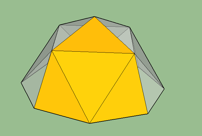
3D Skymap (p=16)
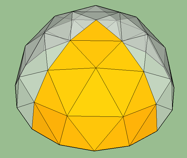
3D Skymap (p=64)
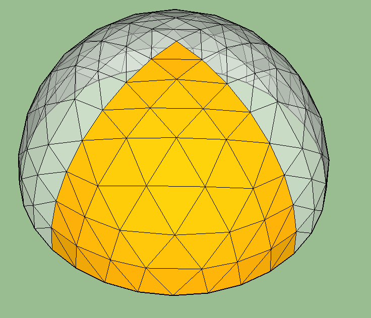
3D Skymap (p=256)
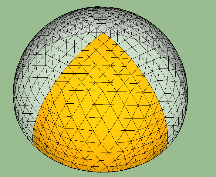
3D Skymap (p=1024)
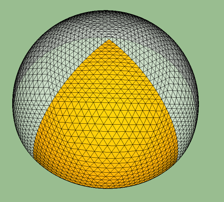
3D Skymap (p=4096)
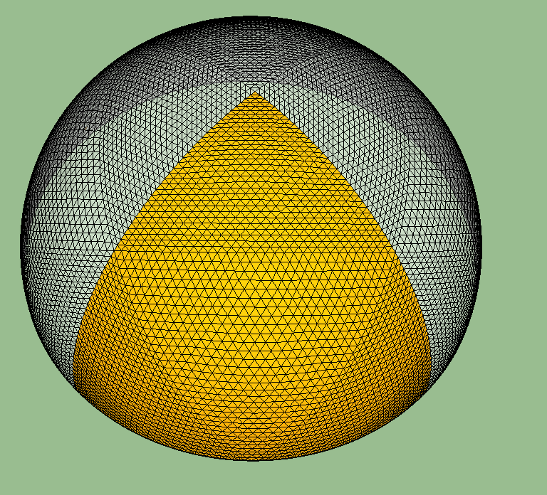
3D Skymap (p=16384)
For n=1, the most basic form is a four-sided pyramid. For n=2, the number of faces is 42= 16. For n=3, the number of faces is 43 = 64 and so on. To calculate running times, each type of 3D SkyView has been repeated ten times, leaving the Ruby Console window on to show the elapsed time after each run. Although computation times will change according to the hardware used, here is a general idea of how long each type of 3D Sky View will take; As you can see, the last construction took 19 minutes (1150 seconds) to finish!
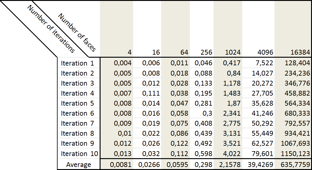
Time (in seconds) taken for each 3D SkyView construction depending on its number of faces
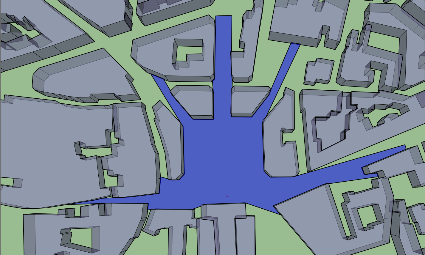
Precision is also important when constructing isovists. As with Sky Views, we have the a choice of 4:sup:`n precision. In this case, we are subject to 4, 16, 64 (...) rays to build our isovist. Too few rays, and the negative space will not be entirely mapped out :
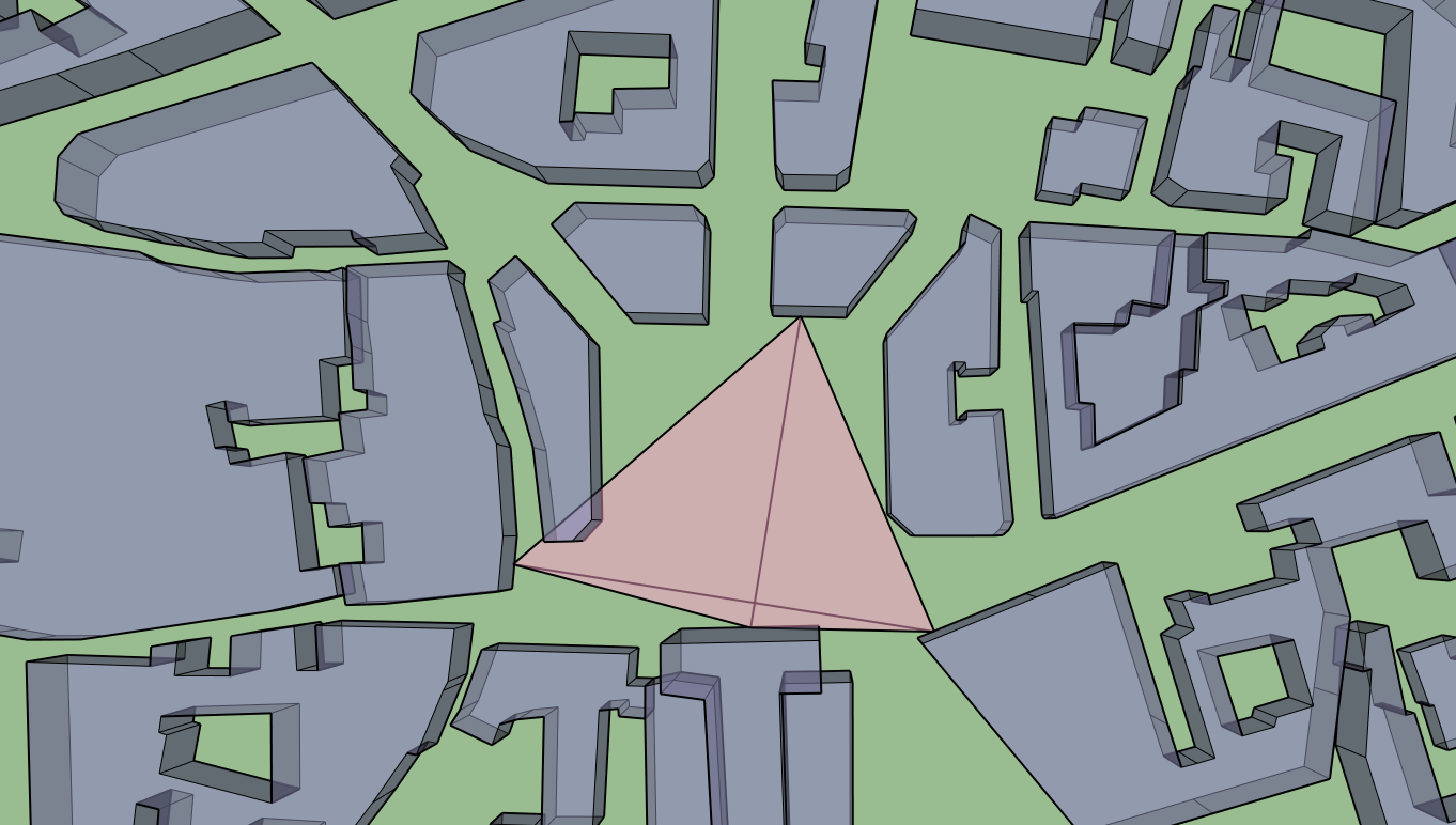
2D isovist built with 4 Rays, also shown.
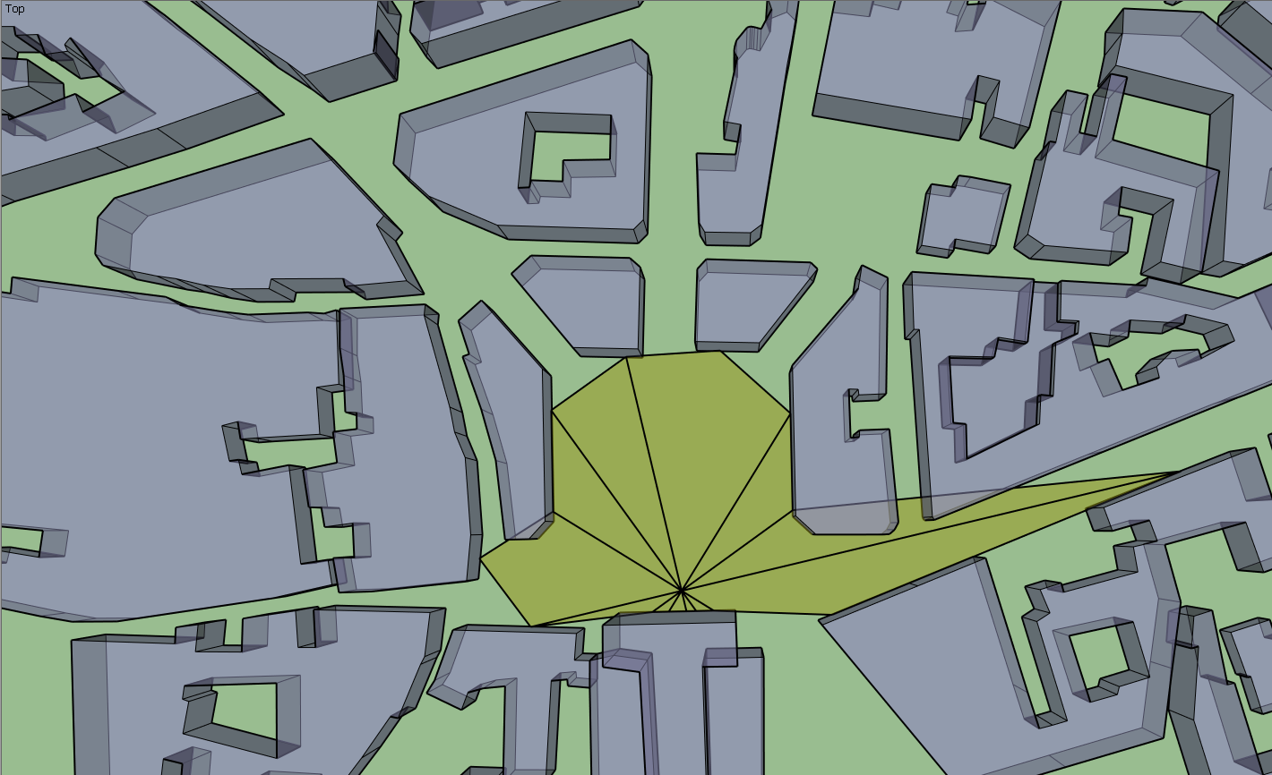
2D isovist built with 16 rays, also shown
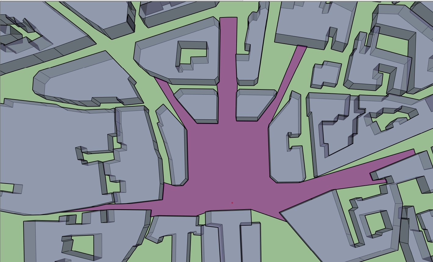
In the pictures above (n=1,2 respectively), because the precision is too low, parts of the isovist traverse the buildings. You can verify this by clicking View > Face Style > X-ray. When moving to a precision of 256 (n=3), we can still notice a small error:
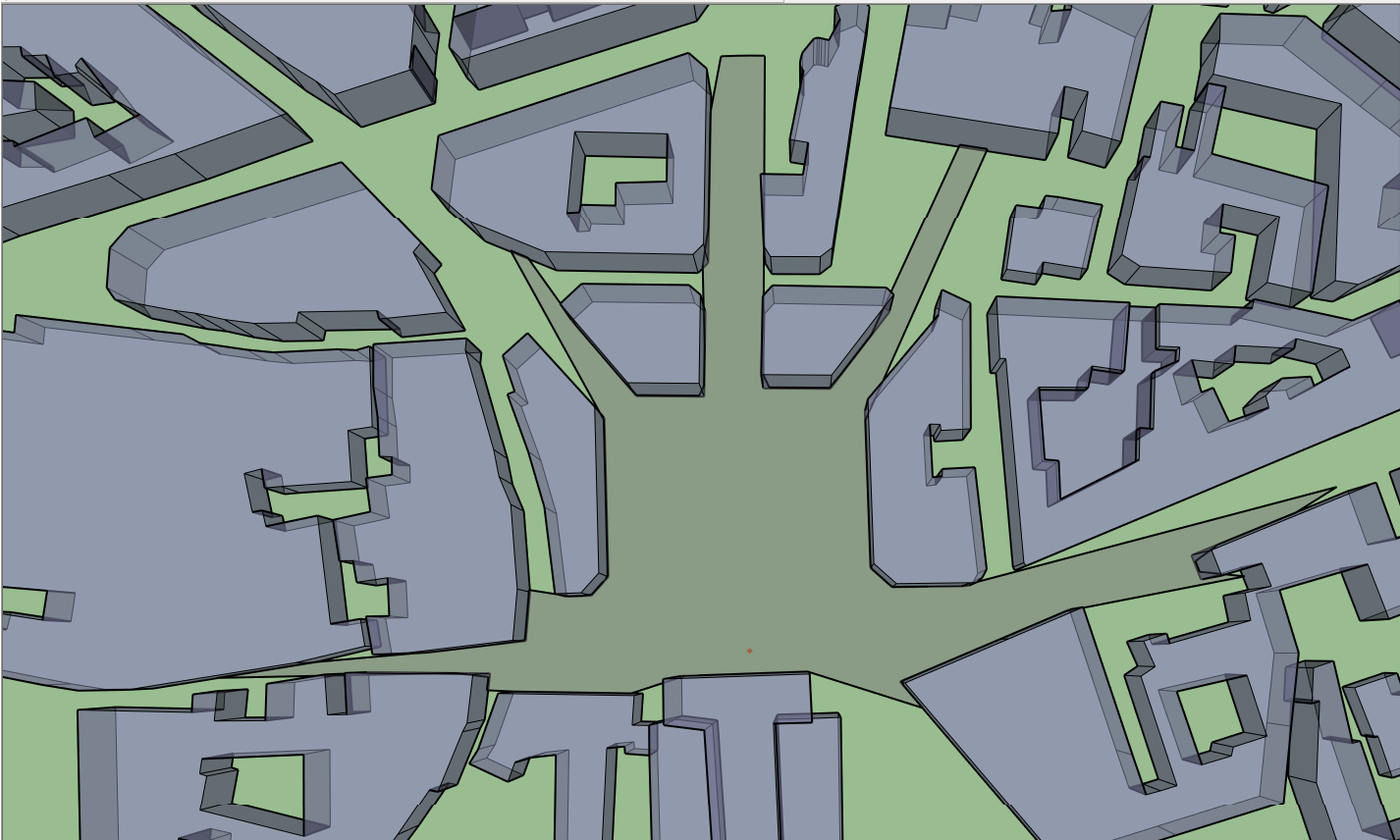
2D Isovist Constituted of 256 Rays.
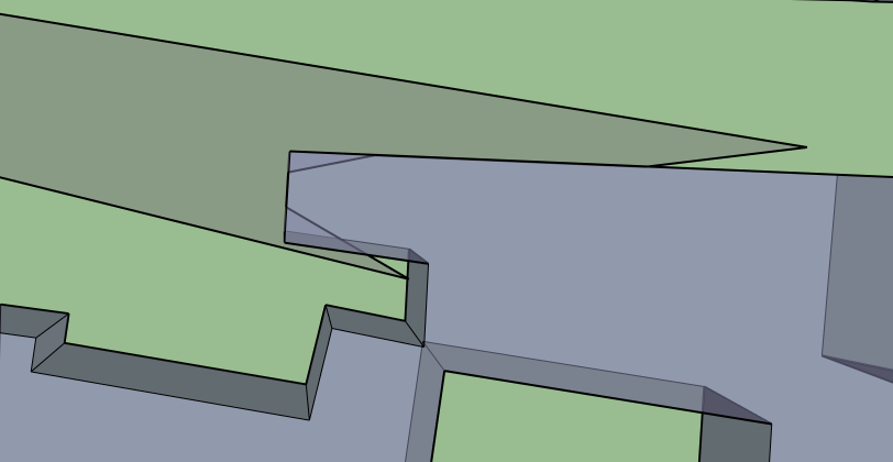
Close-Up of the 256-Ray Isovist.
Moving to 1024 or 4096 rays correct this problem: they are almost identical, but the first one takes approximately 0.3 seconds whilst the second one take 1.3 seconds.
2D Isovist (1024)
2D Isovist (4096)
In this case, the isovist with a precision of 1024 rays has the best precision to calculation time ratio.
See also
5.4. Using Buffers as Visual Information
T4su allows you to create buffers around points: a polygon enclosing a point at a fixed distance. You can access it by clicking Extensions > t4su > Edit > Buffer.
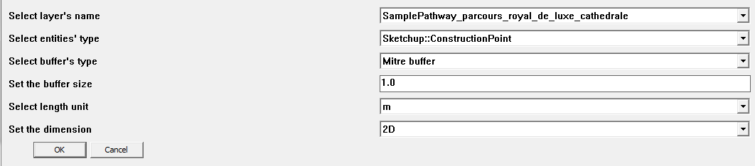
The buffer’s form can be either Round or Mitre, meaning square.
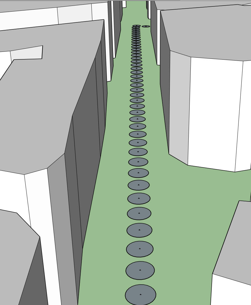
Round 2D Buffers
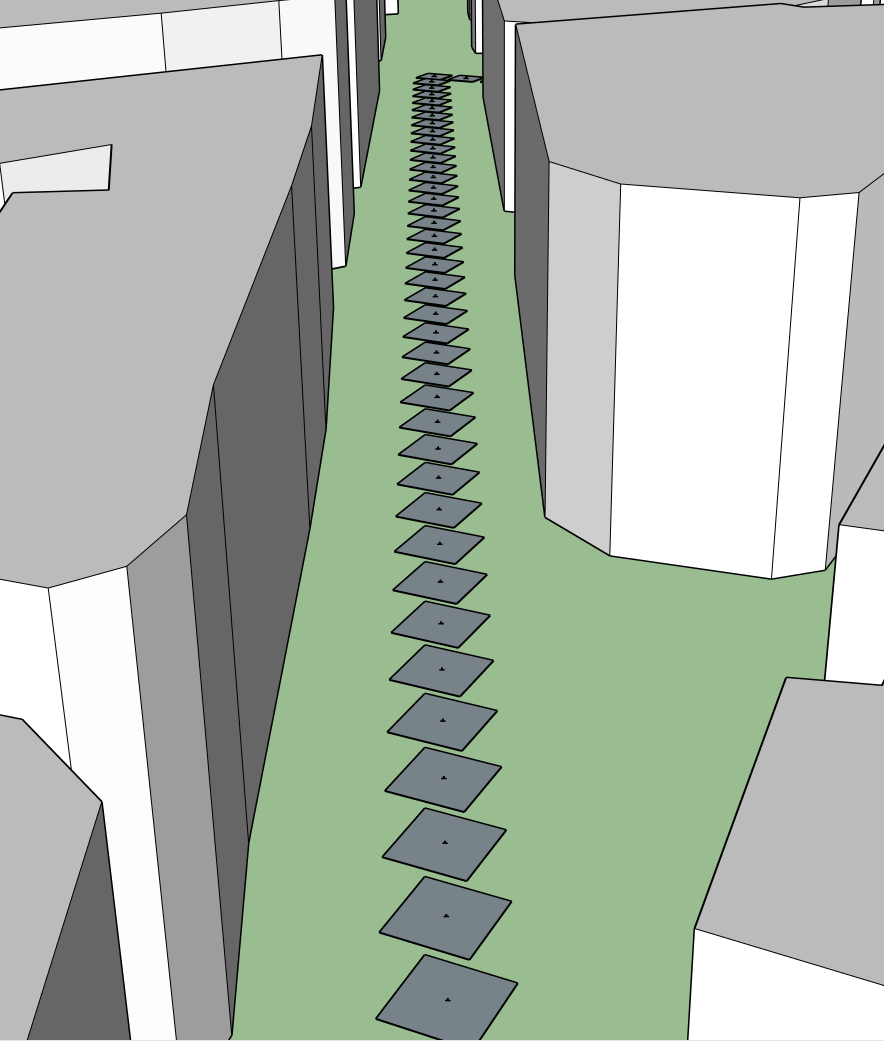
Mitre 2D Buffers
The buffer’s command box also allows you to set your buffer in 2D or 3D space. If you have selected a mitre buffer, the 3D result will be a cube, the size of the sides being your set buffer size. If you’ve selected a round buffer, your set buffer size will represent the length of the radius of a sphere.
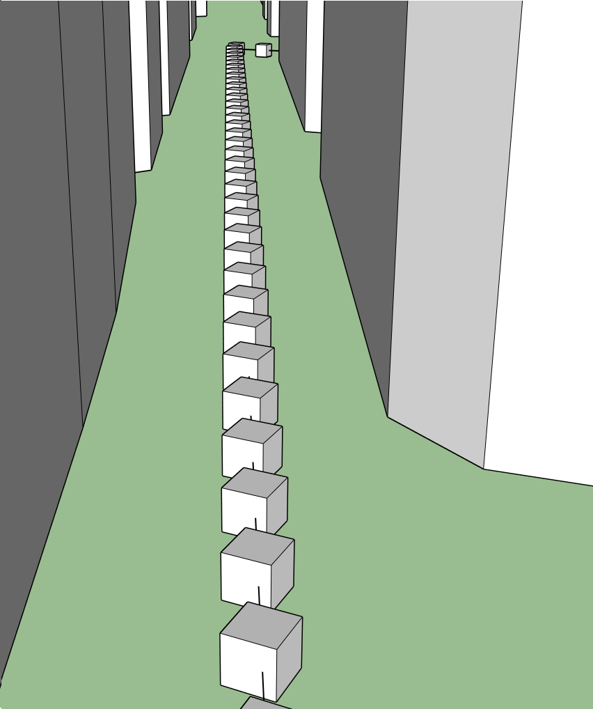
Cubic Buffer
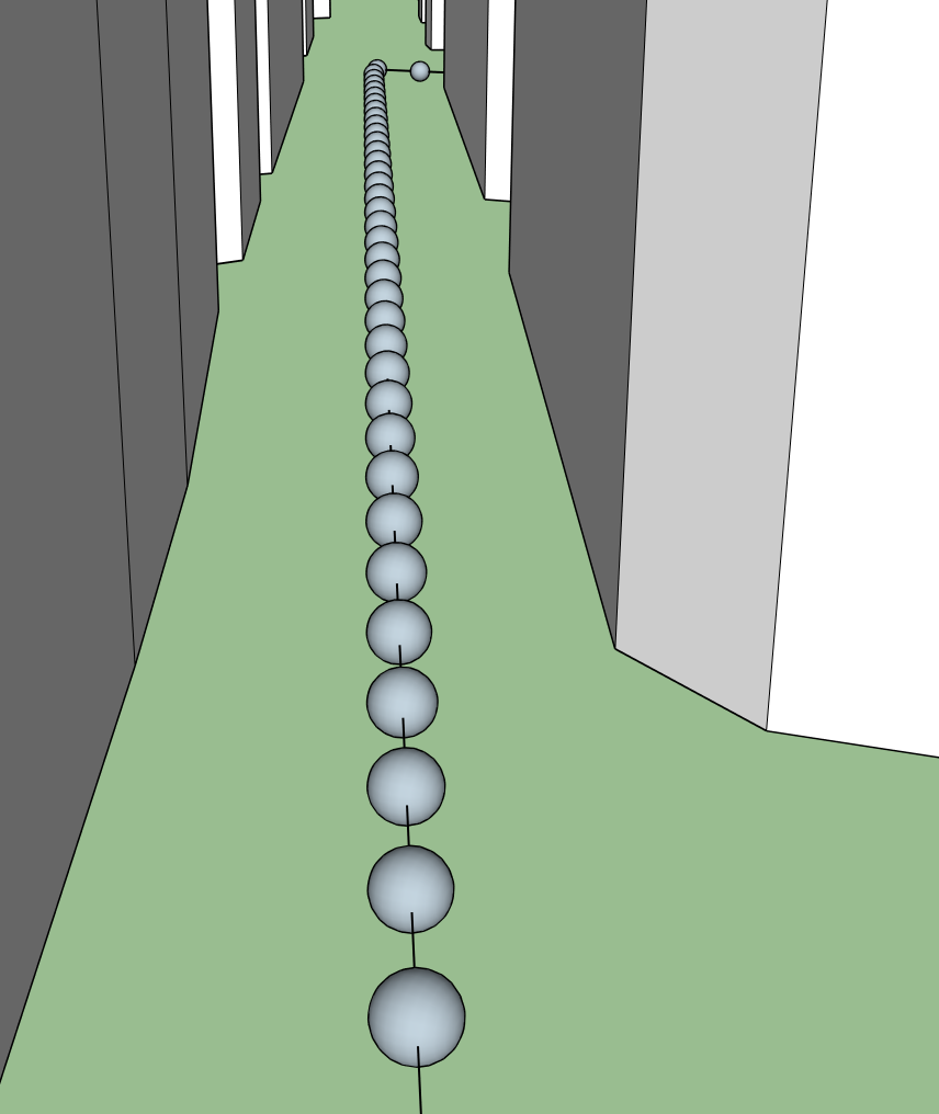
Spheric Buffer
Warning
These buffers are regular geometries in your field. If they are left apparent while running a module that requires ray casting, your buffers will be taken into account and will interfere with the calculations.
5.5. Basic Example of Data Visualization
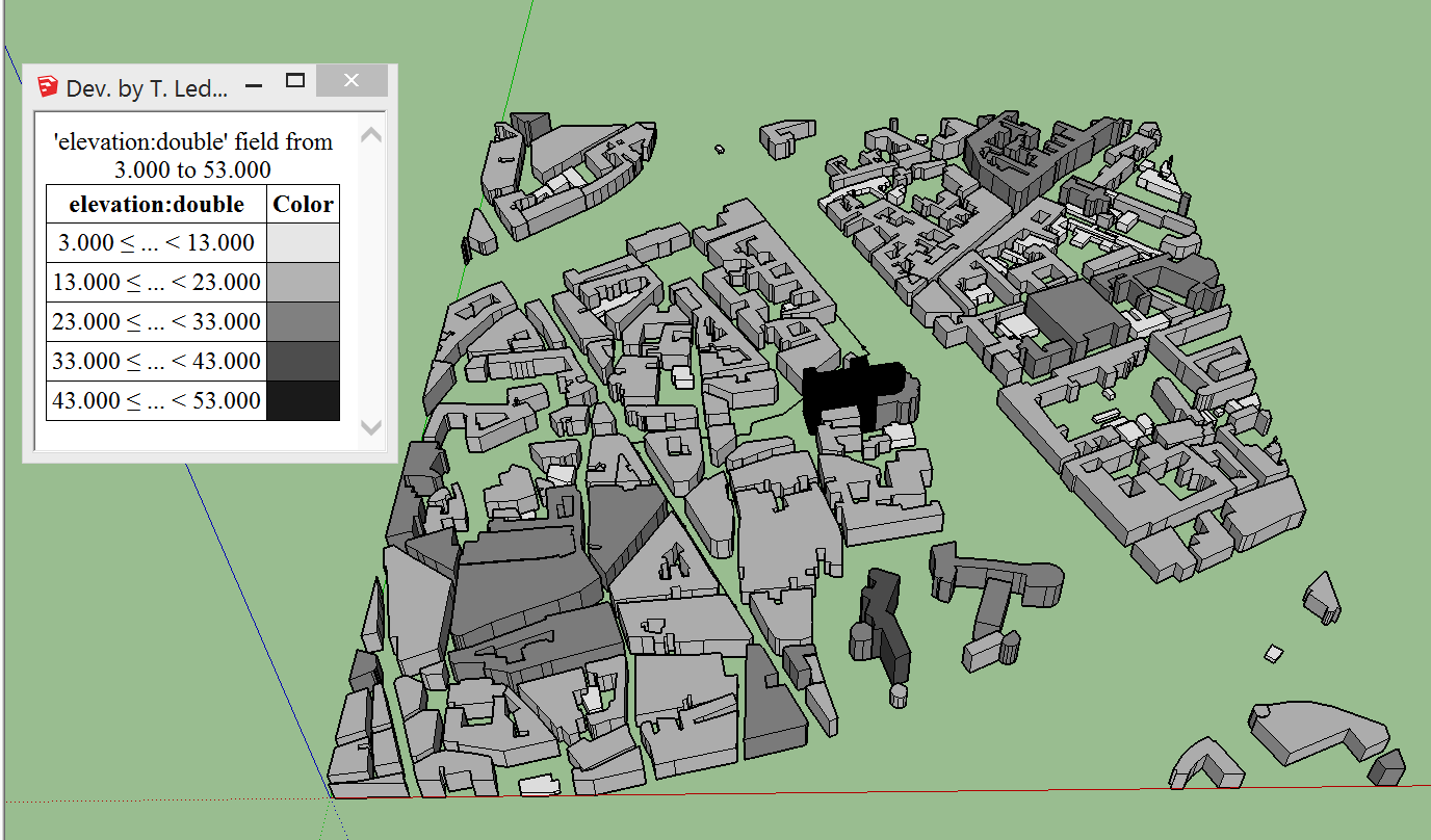
T4su allows for an easy and rapid way of determining the range of building heights.
First, click Extensions > t4su > View > ColorFaces
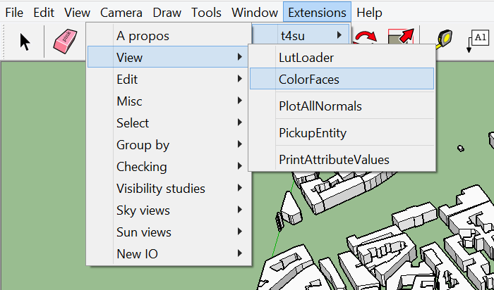
The following box will appear :
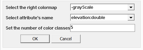
- Select your color scheme. You will notice that all colors appear twice, one of each containing a “-” in front (see picture above). Selecting a color scheme without “-” will allocate darker colors to smaller buildings and lighter colors to taller buildings. The “-” will produce the opposite : darker colors for higher buildings, lighter colors for smaller buildings.
- Select the correct attribute amongst the list. Here we have selected building heights (elevation:double) but you could choose another criteria ( as long as it is float or integer).
- Select the number of classes you wish to create. This is entirely up to you, but keep in mind that above 5 classes, the difference in color may be difficult to distinguish. If you do, we recommend you use “fire”, “ice” or “GreenRed” which allows for a change of hue instead of a change in lightness / darkness. Be careful to select a color scheme that corresponds to the nature of your data.
Here is an example of the end result :